Algorithm Analysis
Asymptotic Notations
Asymptotic notations are the mathematical notations used to describe the running time of an algorithm when the input tends towards a particular value or a limiting value.
For example: In bubble sort,
- when the input array is already sorted, the time taken by the algorithm is linear i.e. the best case.
- But, when the input array is in reverse condition, the algorithm takes the maximum time (quadratic) to sort the elements i.e. the worst case.
- When the input array is neither sorted nor in reverse order, then it takes average time. These durations are denoted using asymptotic notations.
There are mainly three asymptotic notations:
- Big-O notation: represents the upper bound of the running time of an algorithm. Thus, it gives the worst-case complexity of an algorithm.
- Omega notation: represents the lower bound of the running time of an algorithm. Thus, it provides the best case complexity of an algorithm.
- Theta notation: Encloses the function from above and below. It represents the upper and the lower bound of the running time of an algorithm, it is used for analyzing the average-case complexity of an algorithm.
Big-O Analysis of Algorithms
We can express algorithmic complexity using the big-O notation. For a problem of size N:
- A constant-time function/method is “order 1” :
O(1) - A linear-time function/method is “order N” :
O(N) - A quadratic-time function/method is “order N squared” :
O(N^2)
Definition
The general step wise procedure for Big-O runtime analysis is as follows:
- Figure out what the input is and what n represents.
- Express the maximum number of operations, the algorithm performs in terms of n.
- Eliminate all excluding the highest order terms.
- Remove all the constant factors.
Constant Multiplication: If f(n) = c*g(n), then O(f(n)) = O(g(n)) ; where c is a nonzero constant.
Polynomial Function: If f(n) = a0 * n^0 + a1 * n^1 + a2 * n^2 + ... + am * n^m, then O(f(n)) = O(n^m).
Summation Function: If f(n) = f1(n) + f2(n) + ... + fm(n) and fi(n) ≤ fi+1(n) ∀ i = 1, 2, ..., m, then O(f(n)) = O(max(f1(n), f2(n), ..., fm(n))).
Logarithmic Function: If f(n) = loga(n) and g(n) = logb(n), then O(f(n)) = O(g(n)); all log functions grow in the same manner in terms of Big-O.
Basically, this asymptotic notation is used to measure and compare the worst-case scenarios of algorithms theoretically.
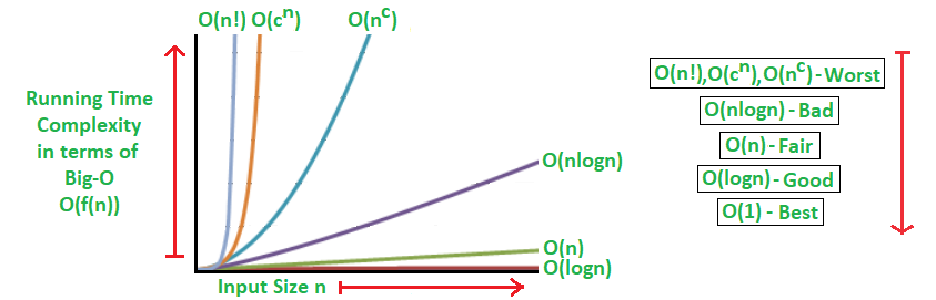
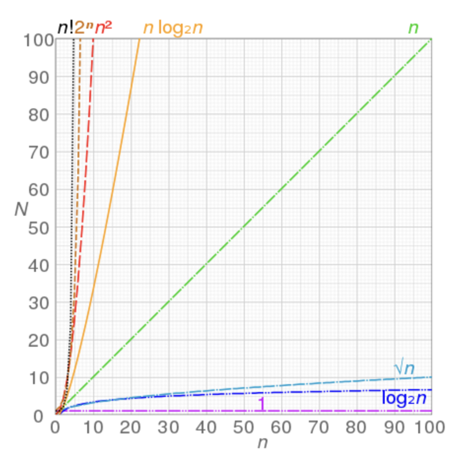
The algorithms can be classified as follows from the best-to-worst performance, (n is the input size and c is a positive constant).:
- A logarithmic algorithm – O(logn): Runtime grows logarithmically in proportion to n.
- A linear algorithm – O(n): Runtime grows directly in proportion to n.
- A superlinear algorithm – O(nlogn): Runtime grows in proportion to n.
- A polynomial algorithm – O(n^c): Runtime grows quicker than previous all based on n.
- A exponential algorithm – O(c^n): Runtime grows even faster than polynomial algorithm based on n.
- A factorial algorithm – O(n!): Runtime grows the fastest and becomes quickly unusable for even small values of n.
For Runtime Analysis, Some of the examples of all those types of algorithms (in worst-case scenarios) are mentioned below:
- O(logn) – Binary Search.
- O(n) – Linear Search.
- O(nlogn) – Heap Sort, Merge Sort.
- O(n^c) – Strassen’s Matrix Multiplication, Bubble Sort, Selection Sort, Insertion Sort, Bucket Sort.
- O(c^n) – Tower of Hanoi.
- O(n!) – Determinant Expansion by Minors, Brute force Search algorithm for Traveling Salesman Problem.
The algorithms with examples are classified from the best-to-worst performance (Space Complexity) based on the worst-case scenarios are mentioned below:
- O(1) - Linear Search, Binary Search, Bubble Sort, Selection Sort, Insertion Sort, Heap Sort, Shell Sort.
- O(log n) - Merge Sort.
- O(n) - Quick Sort.
- O(n+k) - Radix Sort.
There is usually a trade-off between optimal memory use and runtime performance. In general for an algorithm, space efficiency and time efficiency reach at two opposite ends and each point in between them has a certain time and space efficiency. So, the more time efficiency you have, the less space efficiency you have and vice versa.
Space Complexity
auxiliary space complexity: is the extra space or temporary space used by an algorithm.